Home Science Page Data Stream Momentum Directionals Root Beings The Experiment
In exploring the Deviational world, we have found that they are always positive or zero. Looking at some higher Deviations we found that, at least in one Instance, that they possessed the Feature of Stratification. In examining the whys and wherefores of stratification we first examined the deviations themselves. The early deviations were found very easily in terms of the first data points. Very quickly, however, because of the absolute value signs in the general formula, we found that even for the First Deviation of the first Data Point that it had three expressions. It was easily apparent that any further exploration in this path wasn't headed for any simplification.
We then derived an equation for Deviational Differences and applied it to some of the lower and simpler deviations. In an intricate derivation, it was found that for the advanced stage (Joke) of comparing the 2nd and 1st deviation, after the first point only, that the graphic representation contained four different states, shown above. We were just getting started when the complication because of the absolute value signs began multiplying like rabbits. We will finish this study of Deviations with the experimental approach. Hooray for computer graphics!?
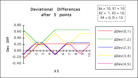
With our initial experimental approach, (Exercise 1976-94), we found that the lower deviations tended to be larger than the higher deviations. In attempting to prove this theoretically, algebraically, we found that indeed this was not always the case. We started at the elemental level and found that sometimes, under special circumstances, the higher deviations were greater than the lower deviations. In trying to find some absolutes, we delved into the content of our equations, by reducing all the higher deviations to functions of X0, X1, & X2. Immediately, because of the multiple conditions imposed by the absolute value signs in the general formula for the difference of deviations, further progress became prohibitive after only the third point. Still hoping for an emergent pattern, we bounced back to the experimental approach. The multiplicity became even greater still. Following is only one of an infinity of different patterns after only 5 points. Already the diversity is incredible. Whenever the lines go beneath the X-axis one of the higher deviations is greater than the lower deviations. There are three blips below the axis in irregular places. Let us throw up our hands at the multiplicity.
At this point in our exploration of deviational differences, we are at a dead end. The reductionist approach, reducing our problem to its most basic elements, had fallen on the rocks because of increasing complexity. Our experimental approach has only reflected more diversity but no overall patterns. Because of the immediate multiplication of complexity due to the multiple conditions imposed by absolute value signs, we had to abandon the algebraic theoretical approach. Now the experimental approach yields equally diverse results. Instead of reductionism to find Rules we must turn to the analysis of context, movement through time, to identify Patterns. We will now return to analyze the general equation in general terms in order to find Patterns maybe but not Rules.
Before moving on, we would like to discuss the dynamics of the Deviational general equation, in terms of the differences between consecutive deviations. Let us take another look at the general equation of deviational differences to understand a little more about the context of the changes. We may not be able to make any absolute predictions about which day it might rain but we can say that it is more likely to rain in winter than in the summer. Following are some notational simplifications. First the difference itself.
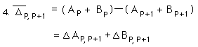
As per our previous treatment, we will break our deviations into A and B parts.
This is the resulting equation of the deviational differences with another notational simplification.
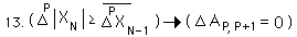
Determining whether our Delta term is positive, negative, or zero will determine whether the lower deviation is >, <, or = the higher deviation.
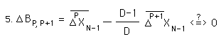
Let us first look at the ∆B term in the equation. Above is its representation. Let us discover the dynamic locked within the symbols.
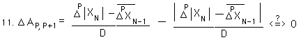
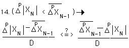
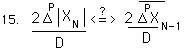
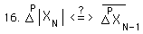
Whichever side of equation #6 is larger will determine whether the ∆B term is positive or negative. If both prior deviations are equal, then ∆B will be positive. The lower deviation must be less than higher deviation by the higher deviation divided by D, the Decay Factor, in order for ∆B to be equal to 0. The lower deviation must be less than this amount for ∆B to be negative. See Equation #7.
For the ∆B term to be negative, the prior higher deviation must be larger than prior lower deviation by the amount specified in Equation #9.
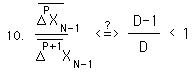
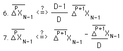
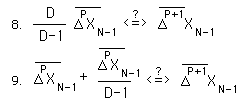
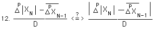
The above ratio expresses the dividing line between greater and lesser. The line is set just below 1. The higher deviation has to be just a little greater to achieve parity with the lower deviation.
The image that arises is of two beings struggling for dominance. One of the beings has a power leak, proportionate to his size. He is operating with a handicap. He is the victim of prejudice. He must be better than the other just to keep up. There is a mechanism that pulls him down. The fight is not fair, because of this mechanism. One is riding with full tires; the other has tires that are a bit deflated. Over the short term the inflation level of the tires doesn't matter so much. The other can exert tremendous energy to win the short-term race. But with each trial, each cycle around the track, the drag of the under inflated wheels takes its toll on the energy and speed of the rider. Falling behind, it is next to impossible to catch up because of this drag on energy and speed. The ∆B element could be called the drag, the friction of the system. In this case it is not linear, but instead proportional to the size of the deviations.
Let us move on to the ∆A component. For simplification we must recollect a definitional equation from the Deviational Change Series.
Applying this definition to the ∆A term, we come up with the following expression.
To determine whether the ∆A term is positive or negative, we need to evaluate the following expression.
When the Pth level of change ≥ the prior deviation of the Pth Deviation, both sides are equal and ∆A = 0. This is expressed symbolically below.
The second condition of the absolute value sign, when the inequalities are reversed, yields the following equation. We dropped the absolute values and reversed the difference.
Combining terms and simplifying, we get the following.
With one last simplification we get the following equivalency.
From Equation #13, we see that when the new change is ≥ to the old average change, that ∆A = 0. As we discovered before, this throws the whole game of which deviation is greater into ∆B's territory, where the higher deviation has a tremendous disadvantage. So whenever the new change is ≥ the old average, the lower deviation gains a tremendous advantage. From Equation #16 we see that whenever the new change < the old average change, then the ∆A term becomes negative. Hence it propels the higher deviation ahead. However even in this situation the ∆B term still operates as a drag on the higher deviation, pulling it down. Furthermore the old average measures an average change, hence, in a stable system, it is just as likely that the new change will be greater or lesser than the old average. With a change in the system that placed the new changes consistently higher than the old average, the lower deviations will steadily gain ground on the higher deviations. This situation occurs when starting a new activity. If the change in the system results in readings, which are consistently lower than the average, then the higher deviations gain an advantage but are still dragged down by the ∆B term. So in an increasing or in a stable Data Stream, the lower deviations will tend to be greater than the higher deviations, (dependent upon past history, of course). While in a decreasing Data Stream the higher deviations gain the advantage. This is the theory behind the Emptiness Principle. {See the Emptiness Principle Notebook.}
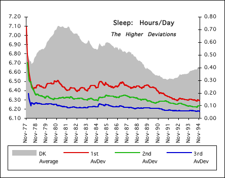
Our first experiment was on an expanding Data Stream – Exercise. Hence it is not surprising that the Deviations stratified in the predicted fashion. Below is an example of a Data Stream in relative equilibrium, Sleep 1977-1994. As predicted the deviations stratify themselves with lower deviations on top and the higher deviations below.
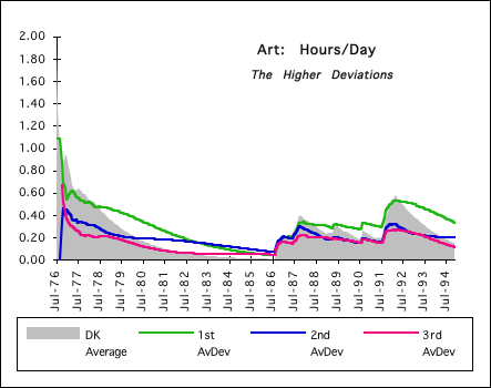
Below is an example of a decreasing Data Stream, (Art 1976->1994). This Data Stream is characterized by extreme activity followed by nothing. In the periods of extreme activity, the deviations tend to stratify. In the periods of decline, the deviations are all mixed up with no predictable stratification, as predicted.