
Home Science Page Data Stream Momentum Directionals Root Beings The Experiment
Before beginning our discussion of Deviations we must look a little more carefully at our foundations. First a distinction must be made between Continuous and Discontinuous Data Streams. A Continuous Data Streams begins from non-existence, hence has a defined history. Many naturally occurring Data Streams begin this way. A baby is born, the beginning of school, to begin playing an instrument. These streams emerge from non-existence. We will call these Continuous Data Streams, because there are no breaks in its history.
There are many other types of streams, which have existed for an indeterminate time before reaching consciousness. Their history is unknown. They emerge into consciousness from a prior existence. We will call these Discontinuous Data Streams because they begin abruptly with no continuous memory. We will begin our Deviational Study with the Continuous Data Stream.
Below is the general representation of a Deviation. P, the order of the deviation, is defined to be an integer greater than or equal to 0. N, the number of samples is normally defined in a similar way. But for the Continuous Data Stream we will define it a little differently.
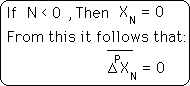
We will define N as any integer, positive, negative, or zero. What does it mean to have a negative number of samples? In this case, the negative samples are the time when our Data Stream didn't exist; hence N is negative. Symbolically this is represented below.
We are not just playing mind games. This makes our first non-zero Data Point, X0. This is the point that our stream comes into existence. It is the real starting point for our stream.
Also because of the non-existence prior to this initial point, our Decay Factor, D, starts at full strength when computing deviations and Directionals. It does not grow with N, the number of samples, until it reaches its full strength, as it does with the other type of stream. The Decay Factor starts at full strength.
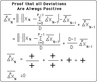
As pointed out above, when N < 0 all deviation = 0. This proof casually shows that every deviation after that is > 0. Therefore, if any deviation = 0 then the Data Stream has not come into existence yet.
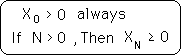
Remember that negative deviations all = 0. Also remember that both X0, the initial point, and D, the Decay Factor, are both > 0. Therefore, with simple algebra, it is easy to see that the first Deviation of the Initial Data Point > 0.
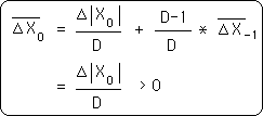
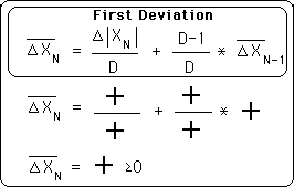
In the simplification below it is easy to see that all the terms that define the first deviation are all > 0. D is defined to be > 0. The ∆|X0| is an absolute value and so is > 0. The prior deviation based upon the deviation before, based upon the deviation before, back to the Initial First Deviation are also all > 0. Thus all the terms that define the First Deviation are > 0.
Therefore when N ≥ 0, the First Deviation is always > 0.
Arguing in a similar fashion it is easy to see that all Deviations are positive. Looking at the general formula for Deviations, we see that the first term is between absolute value signs and so is either positive or zero. The Decay factor, D, is defined as positive. Getting down to more intimate details: the prior deviation can only be negative if the prior deviation is negative, and so forth until we reach the first term of the Pth deviation series, which is always positive because the zeroth term of the Pth deviation always drops out. Therefore there is no way that any deviation could become negative because they are always made up of the sum of positive terms.
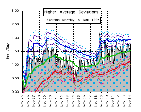
First let us look at some graphic representations of the deviations. Following is a graph of the higher Average Deviations. It is based upon monthly data accumulations for Exercise. The gray background is the real data. The green line represents the Decaying Average, the zeroth Deviation. The thick red line below and the thick blue line above represent a distance of two Average Deviations from the Decaying Mean line. The thinner purple and brown lines are one 2nd Deviation ± from the 1st Deviational line. The dotted light blue and pink lines are one 3rd Deviation ± from the 2nd Deviational line. As can be seen, these Deviational lines represent how much the deviations before them wiggle and wobble.
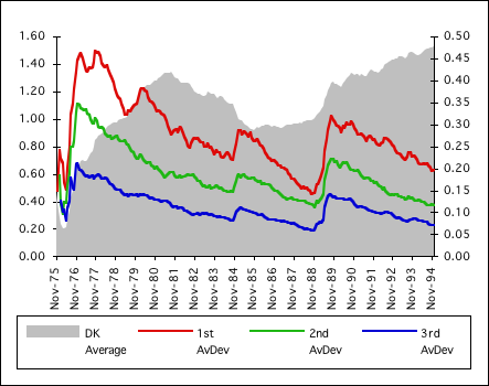
Below is the graph of the Deviations, 0 through 3, from the above graph. The gray background is the zeroth Deviation, the Decaying Average. Its scale is on the left. The red line is the first deviation; the green line is the second deviation; the blue line is the third deviation. It is easy to visually see that the Deviations mimic each other, rising and falling, simultaneously, exclusive of the beginning adjustments and the zeroth Deviation, the Decaying Average. Generally from this graph it would seem that the second and third Deviations offer little new information. They reflect the first deviation rather than yielding new information. The Decaying Average and the First Deviation yield unique information, while the others offer very little that is new.
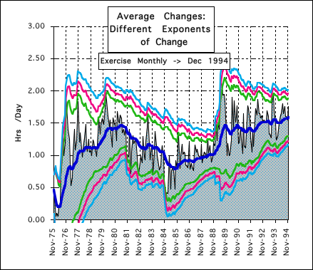
In the previous notebook, Decaying Averages, we introduced the exponent of change. Below is a representation of three different levels of change. The gray background is a representation of the real data. The thick blue line in the middle is the Decaying Average. The green line is 2 deviations away from this average with an exponent of change equaling 1. This is the Average Deviation. The red line is 2 deviations away from the average with an exponent of change equaling 2. This is the Decaying Standard Deviation. The light blue line is 2 deviations away from the average with an exponent of change equaling 3. It is easy to see that each of these Average Changes mimics each other. As the exponent of change gets larger, the average change gets larger. Again the higher exponents of change yield no new information.
The first graph of the series, the Higher Average Deviation graph, is a graphic representation of what the higher Deviations represent. They represent the potential for change of the deviation just below it. As such the first Deviation represents how much the Decaying Average is likely to wobble. Two of these Deviations away from the average on either side, plus or minus, are the boundaries of the Realm of Probability. The second deviation represents how much the first deviation is likely to wiggle. So practically speaking, it extends the boundaries of the Realm by a little. Subsequently the third deviation represents how much the 2nd deviation is likely to wriggle and as such it extends the boundaries of the Realm by a little more. The second graph of the series shows how the higher Deviations are only a reflection of the lower deviations and so don't add much information. Effectively the higher deviations merely increase the boundaries of the realm of probability, but do not yield any unique information of their own. The final graph shows three different Average Changes with different exponents of change. Again each higher exponent of change merely increases the boundaries of the Realm of Probability by a little, but again adds no new information.
Because of the built-in imprecision of a Living Data Stream, it would be very difficult to determine which underlying phenomenon caused the additional wobbling of the boundaries of our Realm of Probability, whether exponential or the higher Deviations. The caveman doesn't care. Only results matter. He varies his boundaries of his Realm from the success of failure of experience, not from the underlying analysis of cause. In this case there is no apparent way to choose between the different causes, because their effects are experimentally indistinguishable. The Effect comes from Indeterminate Causes.
If we were talking about precise physical phenomenon, it might be possible with a series of precise physical experiments, that scientists are known for, to pin down an exact exponent of change, or perhaps to determine how many of the higher deviations to calculate in order to best predict the boundaries of the Realm. But we are talking about Living Data Streams, which are unpredictable by definition. We only need a rough idea of what to expect because of the uncountable number of the other variables that go into making accurate predictions.
Our caveman would not waste his brain space calculating either the higher Deviations or the Deviations with the higher exponents of change. (Why mess with square or cube roots when he doesn't have to.) He would keep it simple. He would calculate his Decaying Average to determine what to expect. He would calculate his Average Deviation in order to know the potential movement of his Decaying Average, the Realm of Probability. With different phenomenon he might experiment with the number of average Deviations from the Average that would include the boundaries of the Realm, but he wouldn't waste his mental time with new measures that merely reflect the information gleaned from his standard measures. Neither will we. Cavemen like to keep things simple; so do we. Henceforth when we refer to the Deviation we will mean the first Deviation with an exponent of change of one.
We have already discovered some characteristics of deviations. They are always ≥ 0. In looking at one graphic Instance of the higher Deviations of a Data Stream, Exercise, we immediately identified a marked Feature, the Deviations stratified from smaller to larger. Is this true for all Data Streams? If not, which ones? If so, why? These questions will be dealt with in the next section. To determine if all Data Streams stratify we will first look at some simple concrete examples. Then to determine why Data Streams have the Feature of stratification we will examine the differences between consecutive Deviations.