Home Science Page Data Stream Momentum Directionals Root Beings The Experiment
In the Momenta diagram above, there are regular holes of improbable possibility. As an example: although there are 24 hours in a day it is unlikely that someone would talk for 24 hours, although' it is possible. If our subject averaged 1.5 hours Talking per day with a SD of 0.35, then the areas of Probable Impossibility would be under 1/2 hour a day or over 2.5 hours a day. Obviously many people talk less than this and many might talk more than this, but for our subject, these are areas of Improbable Possibility. The area of Improbable Possibility for Random Number Streams always equals zero, because there is an equal chance that the Random Number will anywhere within the Range.
The Derivation we are about to see for Data Stream Density is more about defining concepts than it is about a sophisticated proof. First let us create some abbreviations for our concepts. Note the concepts of Data Stream Density and Improbable Possibility. These are the key concepts being dealt with. An understanding of them is crucial to the proof.

In this proof the definitions are the proof. Naming the problem solves it. The upper limit of the Realm of Probability, HiProb, equals three standard deviations above the mean average. The lower limit of the Realm of Probability, LowProb, equals three standard deviations below the mean average. This is the Realm of Probability.

(The three standard deviations is an arbitrary choice. We could just as well have chosen 4 SD, 2 SD, or maybe even 2 Average Deviations, depending upon the constraints of the experiment. We are merely defining the probable area that the Data might fall within.)
The size of the Range equals the difference between upper limit of possibility and the lower limit of possibility. The size of the Realm equals the difference between upper limit of probability and the lower limit of probability, as defined above.

The size of the area of Improbable Possibility is all the space not included in the Realm but included in the Range, i.e. possible, but not probable data values. This is the key definition. The greater this area is, the more tightly contained the probable data values are, hence the greater its density. Conversely, the less this area is, the more diffuse is the realm of probable values, hence the less the data's density.

Hence we define Data Stream Density as the ratio between the area of Improbable Possibility and the Range of Possibility. The Range is fixed. As the Realm becomes smaller, the area of Improbable Possibility becomes larger approaching the Range. Hence the Data Stream Density approaches one. Conversely as the Realm becomes larger, approaching the Range, the area Improbable Possibility gets smaller and the Data Stream Density approaches zero.

Now comes the mini-derivation of a working equation for Data Stream Density. We just use some definitional substitutions and some algebraic manipulations. The area of Improbable Possibility is the difference between the Range and the Realm. The Realm is the difference between the Upper and Lower Limits of Probability. These limits are determined by a certain number of Deviations from the Mean. In this case we have chosen 2 Standard Deviations. The Average cancels out.
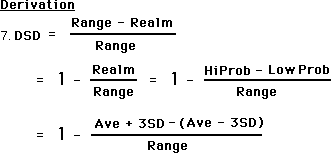
And now the Working Equation of Data Stream Density:

Notice that the Data Stream Density is a function of Range and the Standard Deviation only. The Mean Average does not play a part except perhaps in the generation of the Standard Deviations.
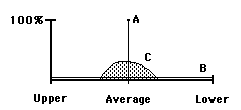
• Line A represents 100% Data Stream Density because all the possibility is concentrated into one point. The numerator of our DSD Equation becomes zero and the equation reduces to one. This is Predestination.
• Line B represents 0% Data Stream Density because any possibility is just as probable. The Numerator equals the Range and the equation reduces to zero. This is Random or Pure Free Will.
• Area C is a mix of the two.
Line A is virtually all Improbable Possibilities because there is only one way and no choice. Line B has no Improbable Possibilities because anything is possible. Line C is a mix. Below is the visualization. The area represents 3 SD + and - the average.
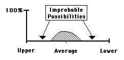
The Data Stream Density is the ratio between the area of Improbable Possibilities and the total area of All Possibilities. When there is no area of Improbable Possibility then the Density is zero. When it is all Improbable Possibility the Density is one.
Strangely enough we must characterize Data Stream Density in terms of what is not, rather than in terms of what is. DSD is the ratio of that which is possible but improbable to all that is possible, see above. With Hard Data or a Dead Data Stream, from the realm of Possible comes only one point that is probable; the rest of the points are improbable. Hence this type of Data Stream has a DSD of One. Conversely, a Random Data Stream where everything is possible and equally probable (no result more or less probable than any other result), there is no area of improbable possibility. Hence the DSD is zero. The Data Stream Density reflects how concentrated or exact the Data is. The more diffuse the data or the stream the lower the density. When the Data becomes more diffuse, it means that there is less improbable possibility. The more exact the number or the predictability of the stream the higher the density. Here the improbable possibility is at a maximum. Therefore the more Improbable Possibility there is, the more exact the Data. The less Improbable Possibility there is, the fuzzier the Data Stream. The amount of Low Probability determines how much High Probability there is and vice versa.
In classic Taoist fashion, Something, Data Stream Density, is defined by Nothing, the Improbable Possibility. On the following page is an Animation, which illustrates the paradox. The first graphic has a Data Stream Density of 0.00. The DSD grows in successive frames. The last one has a Data Stream Density of 1.00. Just as the single Line/Point has a DSD of 1.0 so does nothing at all. Only one course is the same as no choices.


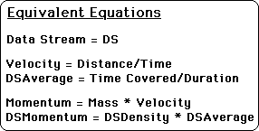
In Physics: Momentum = Mass * Velocity. Momentum is a type of inertial measure since velocity is relative to reference frame. The Velocity of our Data Stream will be equated with its Average. The Average = the Velocity. {Eventually we'll see that it will in fact be the Decaying Average. See Decaying Average Notebook.}
Velocity = Distance/Time. Distance in our case is the number of hours covered each Data Reading. The Time is the Duration over which each Data Reading is taken, i.e. 6 hrs/day, 200 hrs/mo.
Mass is equivalent to the Data Stream Density of a Data Stream. Mass measures the resistance to change. Data Stream Density equals the Improbable Possibility/ Range of Possibility (see above). The Data Stream Density reflects the range of values that our Data Stream wants to stay between. Our Data wants to remain within these boundaries and so also Data Stream Density measures a resistance to change. Below is a summary of these parallels.
How does this relate to anything? We have now defined Data Stream Density and Momentum. What does it mean? Why did we spend so much time defining and refining this concept? We have tried to establish that the momentum of the Data Stream has a life of its own, independent of the Source. Hence in terms of Spiral Time Theory, this momentum is a factor in determining behavior.
In one view, we have no choices. Either divine law or natural laws, a combination of heredity and environment, predetermine all of our behavior. Heredity would be our genetic code with its predispositions. Environment would be the forces at work around us, primarily family and society. In some interpretations the Momentum of the Data Stream would be an environmental factor, which tends to lock us in to preset behavior. This would be certainly true of Dead Data Streams. Because functions rule Dead Data Streams, not data, there is no possibility of breaking out of a Dead Data Stream. Many scientists, especially those studying complicated Dead Data Streams, believe that all phenomenon, even human behavior, is ultimately reducible to the concrete functions of Dead Data Streams.
We, however, believe in the spontaneity, the unpredictability, of Live Data Streams. Furthermore we believe that human behavior generates Live Data Streams with all the inherent unpredictability. Hence, although the momentum of the Data Stream carries behavior along, at any moment there may be a Quake, a discontinuous disruption of the Flow, which will send behavior off in another direction, generating a different type of Flow.
The Flow is the complex of derivatives surrounding a Data Stream. For distinct periods of time, these derivatives stay within a certain boundary. At certain times the Data in Live Data Streams, and as a consequence the Derivatives, will veer substantially from the original Flow. This concept will be dealt with more thoroughly in subsequent Notebooks.
In another view, choice is everything; nothing is predetermined. Humans have an infinity of choices and a 'free will' to choose any of them. Traditional moralists believe that man is faced with the choice of good or evil. If he chooses good, then he should be rewarded. If he chooses evil, then he should be punished. If he is punished for doing evil and rewarded for doing good, then man with his 'free will', in his capacity for choice will choose good. In order to avoid punishment there is the threat of punishment. Because of pure free will, the good man will choose good, while the evil man will choose evil. Here instantaneous conversion is a reality because the 'good' idea can change a man's life, so that he will from henceforth choose good. Because his 'will' is free from the past and only dependent on 'thought', he will only choose good if he is good.
We however also believe in the inherent momentum of Live Data Streams. Remember that Dead Data Streams have a density of one, which ultimately represents only one choice, hence no choice. Random Data Streams have a density of zero; hence they have no momentum at all. Live Data Streams have a Data Density between zero and one. They have enough variety that they can't be pinned down by functions They also have enough order, patterning, that they also exhibit momentum. While Live Data Streams are unpredictable, on all levels, they also exhibit enough of a pattern for momentum to exist. Remember that momentum is based upon the product of Data Density and Average. If there is no pattern, then the Realm of Probability equals the Range of Possibility and the Data Density equals zero. If the Data Density equals zero then the Data Stream has no momentum. It is Random. Only Random Data Streams have a momentum of zero. Only Dead Data Streams have a Density of one. So a Live Data Stream has a Momentum but does not have a Density of one.
Hence although 'will' certainly plays a part in behavior, it would in no way be called 'free'. It might instead be called 'conditioned will'. At any time a being may change his course by will, but there are heavy pressures from the past. These pressures from the past create patterns in the present. These patterns have their own momentum.
It is easy to tell a Random Data Stream from a Live Data Stream. Find the Average. Find the Standard Deviation. If the Average plus 2 Standard Deviations in either direction puts one outside the Range of Possibility on both sides, high and low, then it is a Random Data Stream. {See Random Averages Notebook.}
It is much harder to tell a Live and Dead Data Stream apart. This is why the Cult of Functions continues to thrive and dominate science. Many seemingly Live Data Streams have been killed over the centuries. Functions have been written which perfectly describe previously indescribable Data Streams. Because this has happened so frequently throughout the ages, there is always a healthy skepticism when someone proclaims a phenomenon unpredictable.
In this situation to refine the moment, we are studying the features of unpredictable Data Streams, which we call Live. The unpredictability is part of the postulates. It is not really open to challenge, because it is one of the foundations of an abstract system that has its own features. It would be like challenging a system that assumed that parallel lines never meet. One could however challenge the theory that the system where parallel lines never meet is the system that we live in. In a similar way, one could challenge the theory that humans generate Live Data Streams. Or on a more general level one could challenge the theory that live things generate Live Data Streams. The question is not whether Live Data Streams exist ideally. The real question is whether the ideal world of Live Data Streams has any application to the real world of Live creatures.
Again there is no question that Live creatures generate Data Streams. If there is consciousness to record then everything that exists has Data Streams of some kind. The first real question is whether Live Creatures generate Live, Dead or Random Data Streams. Most humans would agree that Live Creatures, at least, seem to generate Live Data Streams. Although some might believe in undiscovered functions, while others might believe in divine predestination, neither would disagree that humans at least appear to unpredictable. Hence whether humans are really predictable or not is secondary to the fact that they appear to be unpredictable. Hence they appear to generate Live Data Streams. Anyone would agree with this.