
Home Science Page Data Stream Momentum Directionals Root Beings The Experiment
We've determined some criteria to accumulate some Data. We've collected some Data. More is coming. We've begun to calculate a central tendency, i.e. the Mean Average. Let us now look at the range of possible values that our Data can be. If our Data is in terms of hours per day, then our range extends from 0 to 24 hours per day. On any given day the Data that we throw in the box could be anywhere between 0 and 24. This is the Range of Possibility. We start accumulating Data. We generate a running Mean Average. We realize from the above reasoning that the longer we accumulate Data that the more stable, the Mean becomes.
This is true whether we are using Real or Random data. For a Random Data Stream, each Data Byte has an equal chance of being anywhere in the Range. Although the Mean becomes more and more stable as N becomes greater, this gives us no indication as to the next Data Byte. It still has an equal chance of falling anywhere in the Range. The Mean of a Real Data Stream is equally ambiguous. It tells us about the next average but doesn't give us any idea where the next Data Byte might be.
If there were a way to predict the range of probable values of the New Data Byte, then the Experimenter would also be able to predict the range of probable values in the New Average. Limiting the realm of probability, not possibility, concentrates the density of the Data Stream. This concentration of the Data is the Data Density of the Data Stream.
In the first section, we introduced Data Density, which has to do with each Data Byte and its relative existence or non-existence. We defined Data Density as the ratio between Real and Potential. This initial definition referred to a two dimensional density, static in time. We have now introduced the term Data Stream Density. This refers to the density of the Data as it moves through time, the stability or inertia of the Flow of the Data Stream. This adds another dimension, Time, to the Data. While Data Density deals with the collection of only one Data Point, Data Stream Density has to do with the flow of these Data Points through Time. Hence it is a three dimensional Data Density that we are now referring to. However we will use the same ratio of Real to Possible to define it. But first let us talk a little more about general concepts.
If there is no concentration of Data then the Density is zero. This is true of Random Data Streams. If the concentration is all at one point then the Density is 1, 100%. Because of the inherent unpredictability of Live Data Streams, the concentration will never be at one point. Hence when the momentum of a Data Stream is one it is a Dead Data Stream, i.e. one that is totally predictable. A Live Data Stream because of its unpredictability will have a Density between zero and one. What number would the Density be if our stable Mean gives us so little information? This leads us to our next topic, the Standard Deviation. Before going there let us connect these concepts with Spiral Time Theory.
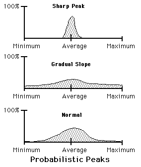
The below diagrams are distribution graphs. The horizontal X-axis represents the Range of possible values that the Data might assume – the lowest on the left, the highest on the right. The vertical Y-axis refers to the percentage of all the data that occurs at the specified position on the X-axis.
Because these diagrams collect a distribution of Data over time and because they limit the probabilities, not the possibilities, of occurrence over the Range, we will call these Time Momenta Diagrams.
In the first diagram 100% of the data falls at only one place. This is a Dead Data Stream. This is the condition of predestination where there is only one choice. One of the underlying assumptions of scientists who believe in a God of functions is that all irregularities can be reduced to this state with a series of transformations. In the second diagram, the Data is equally likely to occur anywhere between Low and High. This is a Random Data Stream. This is also a condition of pure Free Will, when any choice is equally likely. Every action is chosen with no weighting. In the third diagram, it is more likely that the Data will occur around the Average and less likely that it will occur at the extremes. This represents a Live Data Stream. This is the condition of Spiral Time when the Data Stream has density, which leads to momentum, as we shall see, but is still not all determining.
As is shown in the diagrams above, Free Will and Predestination are orthogonal, perpendicular, to each other. Spiral Time, however, links the two in a merger of Flow and Will. With predestination there is only one way. With Free Will, anything is possible. With Spiral Time there is a greater likelihood of one thing happening than another, but nothing is predetermined. The next Data Point is most likely going to be in the middle but it is possible that it could also pop out at minimum or maximum. Traditional hard science deals only with the first possibility, that all physical behavior is predetermined. If variation exists, they look for another variable to cover the variation. Einstein's great achievement was that he discovered a series of equations to absorb more of these variations or wiggles.
Following are three different types of probabilistic time Momenta. In the first we have a very sharp peak with many values excluded for all practical purposes. In the second all values can occur but some a little more likely than another. The third diagram shows the typical Normal Distribution with the most in the middle and with less and less towards the extremes.
Each of these diagrams is two-fold. At one level they represent the data distributions in different Streams. On another level they represent probabilistic predictions for the next Data Bit.
Below is a Diagram of the Momenta of 4 consecutive pieces of Data. Here they are identical. In Reality they change slightly each time based upon the addition of the most recent Data Bit. If the Data Bit is near the center then the edges of the momentum blips are pulled in. If the Data Bit occurs nears the edge, then the center is pulled down or up depending upon which edge. There is no such thing as equilibrium. {See Notebook on Instability Principle.}

The bottom 2 diagrams show the absolute predictability or unpredictability of predestination or a completely free will or random approach. In both of these worldviews, there is no variation, either an infinity of choices or only one choice. Note that only in the top diagram is there any variation.
What measure defines the probable, not possible, variation of our Data Stream? This is where the Standard Deviation, SD, comes in. The SD is a Data Stream measurement, which describes the probability distribution of the data, hence the density of the Data distribution. It is descriptive but it is also predictive. It predicts the potential for variation of the next Data Bit. The SD is based upon the sums of squares.
Each Data Stream has an average. Also each Stream has a Standard Deviation, SD. This is another type of central tendency. This central tendency measures the potential for variation from the mean. 68.26% of the Values of the Stream will be within 1 SD of the average. 95.44% of the Data Bits will be within 2 SD of the Mean and 99.74% of the Data within the Stream will be within 3 SD of the average. The accuracy is based upon the number of samples and the type of distribution.
While the Mean Average and Standard Deviation are descriptive measures, they can also be ascribed predictive capabilities as well. If an individual has averaged between 6 to 7 hours of sleep/per day/per month for 8 years there is a 99% chance he will average between 6 to 7 hours sleep in the next month. There is always a chance that the individual might die in that next month, in which case his Sleep will fall to 0 or rise to 24 depending upon how the experimenter defines Sleep. Probabilistic functions do not define certainty; they define probability. Most scientists use this type of reasoning in making predictions. If a large enough sample has behaved a certain way for a long enough time, then the scientist will make predictions for future values of the set within certain limits. This is not at all controversial.
The average and SD places probabilistic limits on possible values for future elements of our Data Streams. With enough Data Points we can make predictions based upon the Averages and SDs of our Streams. Once again the success of our probabilistic predictions is based upon the number of Data Points, N. The prediction would be that if N is large enough, 99.74% of the new members of the Stream will be within 3 SD of the average. As descriptive measures the central tendencies describe the elements of the Data Stream. As predictive measures they predict the probabilities that the new elements of the Data Stream will fall within certain limits. Within probabilistic limits potential values of a new data point are also limited.
Under the ideas of Pure Will or of Predestination/ 'God as Prime Mover', this probabilistic concept has no meaning, because either the person is unbound by the past or is totally determined by the past. Under the idea that we are influenced by the past but still have a certain free will to choose within the limits of our heredity and environment, these probabilistic predictions attain great significance. The Data Streams actually attain a life of their own, as we shall soon see.
Once we have a Data Stream, we automatically have measures that will make probability projections for the next Data Bit. These measures also make predictions for the Random Data Stream. Ironically these measures predict that the next value of the Random Stream will fall within the limits of possibility and just a little bit beyond. Even Mother Mathematics hedges her bets.
A Random Data Stream has an average, which is most likely to be found in the middle between the possible outer limits. The standard deviation is most likely to be between 3/10 and 1/4 of the range of possible values. {See Random Averages Notebook for theoretical justification.} Therefore 2 Standard Deviations from the Mean Average would extend to a little beyond the upper and lower most limits: just a little beyond the realm of possibility.
For a Random Data Stream, no value in the list of possible values is outside the range of probability. Hence the density of the Random Stream is zero. Let us look at Sleep. The Average for the Sleep Category is 6.7 hours of Sleep a night per month. The SD is 0.13. Therefore there is a 99.75% probability that the next Data Bit in this stream will fall between 6.3 and 7.1. Remember also that these numbers are independent of source. This Data Stream could be referring to any phenomenon and the conclusions would be the same. The Momenta for the Random Stream includes the entire Range and so is quite meaningless while the Real Data Streams just take a little bite out of the 24-hour range. Our individual could possibly sleep between 0 to 24 hours in a day, but will probably sleep between 6.3 and 7.1. The Data Momenta for Sleep are quite tight.
If there were only Dead Data Streams {See Live & Dead Data Streams Notebook for more} then our Data would always fall within its limits. If there were only Dead Data Streams then this whole study would be meaningless for there would be only one choice. But since this study is primarily interested in Live Data Streams, the Data will regularly make erratic jumps beyond the limits of its possibility Momenta. We will call these erratic jumps, Quakes. More on this later.
The Standard Deviation of a truly Dead Data Stream is always zero. Most Streams are a combination of Live and Dead Data Streams. If the scientist even believes in Live Data Streams (many don't) he will still try to concentrate primarily upon data, which is more dead than alive. (It's the fashion right now, especially in the last century.) But the more alive the Data Stream is, the more likely it is to have big jumps, outside the bonds of the Standard Deviations limits. Because of this unpredictability, these Quakes, most scientists prefer Dead Data Sets. Streams are scarier than Sets because they keep on growing. Live Data Streams are even worse because they never behave. The search for predictable functions is futile for Live Data Streams. Thus 'real' scientists laugh at Live Data Streams to hide their abject horror and terror of the Unknown.