A Closer View of the Dynamics of the Living Algorithm's Digestive Process
In prior articles we explored the common dynamical structure that both material systems and the Living Algorithm System share. We first examined where they converge and then in the most recent article where they diverge. This refinement process enables us to more fully differentiate the two systems. We can now begin to integrate the dynamical constructs associated with the information contained in data streams. Let us further refine our understanding of data stream dynamics by digging even deeper into the Living Algorithm's process of digesting information.
Review: Material Systems, Static Information: Living Algorithm System, Dynamic Information
Reiterating to reinforce memory: material systems and the Living Algorithm's information system participate in the same dynamical structure. However, the information in material systems is static, while the information in the Living Algorithm System is dynamic. With this fundamental difference in mind, let's take a closer look at the dynamics behind the Living Algorithm's Digestive Process. We will begin our analysis with an examination of what happens when a series of data bits (1s) enter the Living Algorithm System.
Living Algorithm's Digestion Method spread Data's Impact over Time
The Living Algorithm's digestion method spreads each data bit's contribution over time. This spreading is in contrast to material systems, such as electronics, where the data bit's contribution is immediate and complete. This spreading creates the interactive feature that yields a system of dynamics with the same rules as physical dynamics. Specifically the data bit's info energy enters the system in a reduced form and then decays in a logarithmic fashion. This decay is due to the Living Algorithm's scaling process.
A. Contribution of Individual Data Bits
To the Living Average
Graph: Contribution of Individual Data Bits to the Living Average
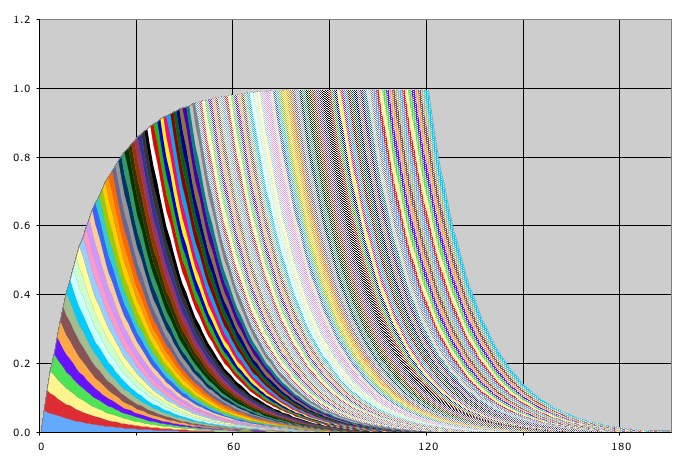
In Graph A at right each color represents an example of what happens when the Living Algorithm digests a single bit of data. These swooping curves gradually accumulate to collectively produce the graceful Living Average curve - the outline of the entire area. The Living Average curve is a picture of the state of the Living Algorithm System at each moment. The graph is a visualization of how much info energy the System is accumulating. In this way, it is like a thermometer, which tells us how much heat energy there is in the room.
The Intimate Relationship between Info Energy and the Living Average
Graph: Living Algorithm spreads data byte's energy over time.
Let's take a closer look at the components of the Living Average to better understand the dynamics of info energy. In the article on Info Energy, we mentioned that info energy is associated with the Living Average. The info energy enters the Living Algorithm System as Raw Data in any form. When the Living Algorithm's Decay Factor is one (D = 1), as in material systems, the info energy is manifested immediately and completely (as seen in the prior article). However, when the Decay Factor is greater than one (D>1) the data's info energy is spread over time. This spreading process is illustrated in the graph at right.
Accumulating Energy does Work of raising the Living Average
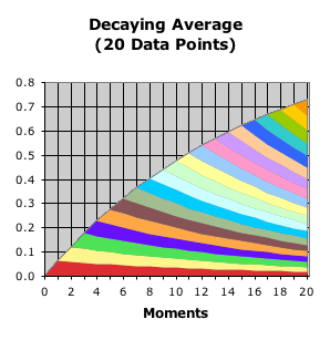
The graph is a picture of the individual contribution of each data byte to the Living Average when the data stream consists of 20 ones. Note this graph is an enlargement of the lower left corner of Graph A (showing only 20 of the 120 ones). Each of the horizontal swatches of color represents the contribution of each data byte's info energy to the Living Average. It is this accumulation of info energy that does the work of moving the Living Average ever higher. Similarly, the accumulation of heat energy in a room drives the thermometer's reading up.
Graph: Individual contribution's of info energy to Decay Average at individual moments.
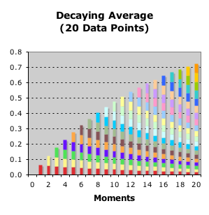
What are the specifics of the process? The data byte’s info energy impacts the Living Average (the state of the System). The size of the initial impact equals the data byte divided by the Decay Factor, D. This is just a fraction of the total info energy contained in the data byte. The rest of the energy from that particular data byte is doled out over time. Specifically, each time the Living Algorithm process is repeated, the amount of info energy that is expended decreases. This doling process is shown in the graph at right.
Doling out Info Energy in Discrete Chunks – Quanta of Info Energy
Each swatch of colored rectangles represents how the info energy behind that particular data bit is doled out. Because of the discrete (not continuous) nature of the energy, we refer to these colored rectangles as quanta of info energy. For instance, the red data byte expends the largest amount of energy at the 1st moment when it enters the System (the red quanta of info energy on the far left). After this initial moment, the quantum of info energy supplied by this data byte and employed to change the Living Average shrinks with each repetition of the Living Algorithm process. This process is seen in the graph. For instance, notice how the initial red quantum is greater in size than the subsequent red quanta, which decrease in size as they move from left to right.
Active Info Energy similar to Kinetic Energy of Material Systems.
The colored rectangles represent the quanta of info energy that is employed at each particular moment. At each moment after entering the System, part of the data's info energy is employed to change the Living Average. In this way, active info energy is similar to kinetic energy in material systems.
Total Info Energy of Data Byte is consumed gradually.
Eventually the total info energy of the initial data byte is completely consumed (at least for practical purposes). We can view the entire process in Graph A at the top of this article. In the current graph, the completion process, although implied, is truncated. When viewing this graphic representation, keep in mind that many more of the scaled info quanta continue inexorably to the right.
Residual Info Energy similar to Potential Energy of Material Systems
The Living Average graph illustrates the energy flow of the System – how much of each data byte’s energy has been employed at any moment and how much info energy remains to be used. For instance, at the 6th moment all of the info quanta to the left on the graph have been employed to change the Living Average. In contrast, all the info quanta to the right of the 6th moment remain to be employed in future moments. All the info energy that has not yet been used is the residual info energy of the System. This residual info energy is similar to potential energy in material systems.
Living Average Grid reveals System's Active & Residual Energy
The graph pictured above is the Living Average Grid. We refer to it as a ‘grid’ because of its visual nature. This particular ‘grid’ reveals much about the info energy flow of the System. For instance, the graph illustrates how much info energy is employed at each moment, the relative size of each quanta of info energy, and when it is expended. Accordingly, we could say that the graph is a grid of info energy quanta.
Living Average reveals little about a Data Stream’s Efficiency and Productivity
An inspection of the Living Average Grid reveals how much energy was expended to change the State of the System and how much info energy remains. In short, an examination of the Living Average Grid tells us everything we need to know about the quantities of info energy. Yet the ‘Grid’ tells us very little about the behavior of info energy - the dynamics of the System. For instance, the ‘matrix’ doesn't reveal how productively or efficiently the info energy was employed.
Must look to Data Stream Acceleration to understand the dynamics of Info Energy
The Living Average, the Living Algorithm’s 1st derivative (rate of change) is the velocity of the System. The 2nd derivative, the Active Pulse, a.k.a. the Pulse of Attention, is the acceleration of the dynamical system. Completing the hierarchy, the Liminals, as a group, represent the still higher derivatives (3rd, 4th, 5th, …). In dynamical systems, we must look to acceleration to understand the behavior of energy – how it manifests itself.
The Accumulation of Individual Accelerations
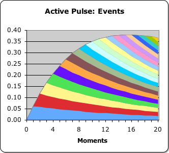
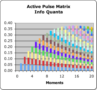
How does acceleration manifest in the Living Algorithm System? The Active Pulse, a.k.a. the Pulse of Attention, is a picture of the acceleration of a string of ones. The Triple Pulse is a visualization of the acceleration of a specific string of ones and zeros. Both of these graphs are composed of the accumulation of the individual accelerations of a sequence data bits. In spreading the impact of each data bit over time, the Living Algorithm's digestive process creates the individual accelerations and the cumulative effect. This process is visualized in the graph at right. Shown are the individual contributions of the first 20 data bits (all ones) to the Pulse of Attention.
Parts reach peak immediately; the Accumulation takes time to reach the peak.
Notice how each individual strip begins at a maximum and then fades. In contrast, the accumulation, the Attention Pulse, starts low, rises to a maximum and then fades. Although both fade out, the individual strips start at their peak, while the Pulse takes some 17 bits to reach its peak. The individual parts and the collective have qualitatively different characteristics. This divergence between the parts and the collective is a good example of emergence.
Data Stream Acceleration Quantized, rather than Continuous
Active Pulse is composed of columns, not curves.
The above graph illustrates the decaying acceleration of each data bit and its accumulating contribution to the whole (the Active Pulse in this case). We chose continuous forms to make a point. However, the visualization of continuous curves is slightly misleading, for the Living Algorithm digests data streams in chunks – info quanta. As such, the Active Pulse curves are not really curves, but are instead a series of columns. Just as an animation is comprised of a series of still pictures that create the illusion of motion, the seeming continuity of the Active Pulse curves is an illusion created by the density and number of columns.
Graphic Visualization: Close-up of Active Pulse as columns
As a way of reinforcing understanding, let's look at a close-up of the result when the Living Algorithm digests the first 20 'ones' of the Active Pulse data stream – the first 20 moments of an 'experience'. (Note: this visualization is based upon the exact same data as the above graph. We just chose a different graphic method to visualize the data. Even the color of each data bit's contribution is the same in the respective graphs.)
Notice how the tops of the columns as a group form the curve of the Active Pulse shown in the earlier graph. This visualization illustrates the fact that the Living Algorithm does not digest a continuous flow of information but instead digests a series of discrete quantities to produce info quanta.
Individual Quantum of Acceleration
Before examining the graph in detail. Let us review what each of the color rectangles represents. The entire graph is a picture of the first 20 moments of the Active Pulse of 1s – the acceleration of the data stream. The Living Algorithm's digestion process spreads the contribution of each data bit over time, not continuously, but incrementally. The entire contribution is doled out gradually in decreasing portions. Accordingly, each of the colored rectangles represents the contribution of the individual data to the entire acceleration at that moment in time. Let's refer to each colored rectangle as an info quantum of acceleration. As is evident, each quantum can be of variable size.
Accumulation of Individual Acceleration Quanta determines the Acceleration of a given Moment
Let's be specific. The blue rectangle over the 1 indicates the contribution of the 1st data bit to the data stream's acceleration at the 1st moment in time. The blue rectangle over the 2 indicates the first data bit's contribution to the acceleration at the 2nd moment in time. The blue rectangle joins with the 1st red rectangle (the acceleration of the 2nd data bit) to yield the total acceleration at the 2nd moment. The blue, red and yellow rectangles (all quantum of acceleration) add up to equal the 3rd moment's acceleration. The accumulation or sum of all the acceleration quantum at each point in time determines the acceleration of that moment.
Attention is the glue that binds Info Quanta.
Velocity and Acceleration are abstractions without Substance
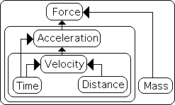
So far this discussion has been a purely mathematical exercise - an abstraction without ties to reality. In similar fashion, physical velocity and acceleration existing alone are purely mental constructs. These material rates of change must be associated with a substance (mass) to exist. Mass combined with velocity yields real world momentum; the acceleration of physical mass yields real world force. Similarly, data stream velocity and acceleration require some kind of substance to tie them to the real world. Attention provides that substance. Attention is focused mental energy, as discussed in the article on Data Stream Mass.
These relationships are shown in the architecture of dynamics. Notice how Mass is required to take Velocity and Acceleration to the next level. Before Mass was introduced, there was no connection to the real world. Attention provides the connection to the world of information.
Attention provides Substance to Data Stream Velocity & Acceleration.
The aforementioned accumulation of acceleration quanta does not occur spontaneously. Mental energy is required. Attention is the glue that binds the stream together. This is why we sometimes refer to the Active Pulse as the Pulse of Attention. As the glue, Attention also provides substance to the data stream. Without Attention, the data stream remains undigested, and its information is transferred instantly and completely to the environment. Only with Attention can the data stream be digested. The digestion process relates the past to the present - providing an accumulated memory of what went before.
Assumption: Attention is binary – 'on' or 'off'
To simplify our discussion, we assume that Attention (mental substance) is binary, either 'on'' or 'off' – 1 or 0. During the Active Pulse, Attention is 'on' and generates 1s. During the Rest Pulse, Attention is 'off' and generates 0s. Without Attention, the dynamic information contained in data streams remains undigested, and as such is meaningless to the organism.
Info quanta (the colored rectangles) are quanta of info force.
Refreshing our dynamics for comprehension: physical mass (substance) combined with acceleration yields physical force. In similar fashion, mental Attention (substance) combined with data stream acceleration yields data stream force (discussed in more depth in the article of the same name). Viewed in this light, our acceleration quanta (the colored rectangles of the Active Pulse) are actually quanta of info force. In other words, the only way that info quanta can become a continuous entity is via the ‘connective’ substance of Attention. Without the connective feature of Attention, the info quanta remain isolated. Sustaining Attention on a data stream is the only way that the accumulation of info forces (colored rectangles) becomes the Active Pulse.
The Power of Attention
Completed Structure of Dynamics includes Work and Power
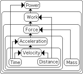
Let us remember our completed structure of dynamics. Note that the dynamical constructs of Work and Power have been added to the architecture. Work indicates Force applied over Distance, like pushing a rock up an incline. Power is how quickly this Work is accomplished over Time. These constructs are intimately entwined with Energy.
Walk or Drive? An everyday consideration of Energy & Power.
To facilitate understanding, let's put a face on these dynamical concepts. We regularly consider the issues of Energy, Work & Power, when deciding whether to walk, bike or drive to a particular destination. We ask how much Time and Energy do we want to invest in walking to our destination compared with the Time and Energy expended in driving and parking our car. Moving one's body or car (Force) over Distance is Work. It takes Energy to do Work. We might consider taking a car if we are tired because walking takes more energy. We consider the issue of Power when determining how much time it will take to reach our destination. If we have plenty of time, we might choose to a slower (less powerful) form of transportation, such as walking. If our time is short, we require a faster (more powerful) mode of transportation.
Mental Energy balanced with Physical Energy
Note: most of us consider the expenditure of mental energy as well physical energy. Perhaps employing our mental energy (Attention) over time (Power) dealing with traffic and parking leaves us drained. Taking this mental drain into account, we might choose to walk a longer distance - expend more physical energy to save our mental energy of Attention. As biological organisms, we have limited resources. Accordingly, we regularly balance mental and physical energy expenditure when making choices.
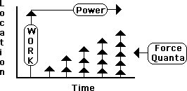
Active Pulse Grid: Vertical Columns represent Work
The structure of dynamics is reflected in the Grid of the Active Pulse (shown at right). Each column represents a moment and how much work is done at that moment. Each of the force quantum (the colored rectangles comprising each column) add up to indicate how much work the info energy is accomplishing at a given moment. For instance, notice that the amount of work accomplished peaks at around the 17th moment. After the 17th moment, the amount of work begins to fade. Remembering the complete curve of the Active Pulse, we know that the amount of work eventually fades to nothing.
Active Pulse Grid: Horizontal Summation of Columns equals Power
We've demonstrated that each column represents a moment in time. The height of each column indicates the total amount of actual work done by the info energy at that moment in time. The columns represent the vertical component of the Active Pulse's Grid. There is no motion through time, just work. When the columns are connected via Attention, we see how much work is accomplished over time. This summation addresses the horizontal component of the Active Pulse Grid. The sum of the columns represents the work accomplished over time. Work over Time is Power. Accordingly, the Power of the System is the combination of the both vertical and horizontal components of the Active Pulse Grid.
The Active Pulse = The Power of Attention
Reiterating for emphasis, the work accomplished at individual moments is the sum of all the force quanta at that moment. In other words, the force quanta of the individual data bits accumulate to indicate the total work performed at each moment. The sum of all the force quanta, both horizontal and vertical, determines the power of a particular data stream. Attention is the glue that binds the Active Pulse Grid. As indicated, the Active Pulse Grid represents the power of the system. Accordingly the Active Pulse could also be called the Power of Attention. (For the algebra behind this analysis check out Info Quanta.)
Data Stream Efficiency
We can now determine the Efficiency of a Data Stream. It is simply Power divided by Total Energy. The Active Pulse's Efficiency (our example) is 15.3%. To calculate this number we first summed up the area under the curve (the columns). We then divided this number by the amount of energy consumed – the total energy (120) minus the residual energy (16) that hasn’t been consumed. In contrast, for a random data stream, the efficiency hovers around 0%, sometimes positive, sometimes negative. In broad terms, we can say that a random data stream lacks any efficiency whatsoever. This result accords with common sense.
Data Stream Efficiency low compared to Physical Systems
Relative to many physical systems, the Active Pulse's Efficiency is low. This is due to yet another significant difference between the Living Algorithm’s information system and material systems.
The amount of energy in closed physical systems is constant. This notion is reflected in the primary law of thermodynamics – the conservation of energy. Descartes was the first to recognize this particular characteristic of matter. From specific examples, he inferred that there is a constant amount of physical momentum in the Universe, and that this amazing equality is a testament to God's almighty glory.
Entropic nature of Living Algorithm
In contrast, the Living Algorithm System is constantly fighting the innate entropic forces of the Decay Factor. Due to the Decay Factor, the state of the System is steadily scaled down. As a result, the incoming info energy is employed to both change and maintain the system. In the second capacity, the info energy is employed to reverse the innate entropy of the Living Algorithm System. In contrast to material systems, this energy does not go anywhere. It is neither dissipated into the greater world, nor does it reduce the organization of the system to which it belongs. It merely disappears. Consequently much of the mental energy behind the Living Algorithm is fighting decay - attempting to reverse entropy.
Graph: Physical Power vs. Data Stream Power
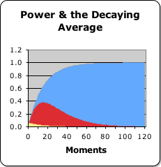
As mentioned, the mental energy of Attention is continuously employed to both change and maintain the state of the System. As an example of how much mental energy is required to just maintain gains, check out the graph at the right. This visual representation compares how much data stream (or mental) power is required to change the system versus power in the traditional sense.
The blue area in the background is the Living Average of a data stream consisting of 120 1s. The tiny yellow sliver at the bottom represents the amount of ‘traditionally’ computed power that it would take to change the system from zero to one. This computation is based upon how much the Living Average changes, i.e. the amount of work done in a given interval. The red area (the Active Pulse) represents the amount of data stream power required to raise the Living Average the same distance. Notice how much more data stream power is required to do the same job. Fighting entropy is not easy, as anyone who cleans a house understands.
Links
We've employed many articles discussing data stream dynamics. What relevance does this intriguing concept have for human behavior? How does it apply? For more, check out the next article in the series - A Continuous vs. a Core Concept Lecture.