Introduction to Information Quanta
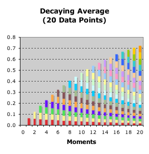
In the article entitled Integration: Living Algorithm Dynamics, we introduced the graph at the left as a way of understanding energy in the Living Algorithm System. In fact, each of the colored rectangles represents a discrete packet of info energy. These information packets enable us to visualize the actual flow of info energy in a data stream. The aim of this article is to derive the value of each of the info packets (colored rectangles). The derivation process will reveal some of the System's invariable mathematical features.
Quanta of Information
Let's begin with the notion that each colored rectangle in the graph represents a 'quantum' of information energy. Webster’s Dictionary defines quantum as “an elemental unit of energy according to the quantum theory of Physics.” Webster’s goes on to define quantum theory as “a theory that in the emission or absorption of energy by atoms or molecules the process is not continuous but takes place by steps, each step being the emission or absorption of an amount of energy called the quantum.”
Photons are Quanta of Light Energy
To better understand the 'quantum' notion let us investigate an example from Physics. White light can be broken down into all the colors of the rainbow. The colors can be further broken down into specific locations on the electromagnetic spectrum. Each of these color locations can be further broken down into a light wave. Ultimately, the light wave can be broken into a stream of photons. A photon is a quantum of light’s radiant energy. As an element unit, a quantum of light energy cannot be broken down any further. All quanta (plural of quantum) of light contain the same energy or momentum.
Color Rectangles are Quanta of Info Energy
Graph: the Living Average & Active Pulse – a Simple Curve
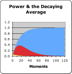
In similar fashion, both the Living Average and the Active Pulse, a.k.a. the Pulse of Attention, can be visualized as simple curves. The curved blue area in the graph at left represents the Living Average and the red curved area the Active Pulse. These curves are the result when the Living Algorithm digests a data stream consisting of 120 ones. The Living Algorithm's digestion process reveals a data stream's rates of change (derivatives). The curves indicate the values of the 1st and 2nd derivatives of a data stream of 120 ones at each moment.
Graph: the Living Average: Horizontal Components – Data Bit's Contribution over Time
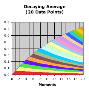
This curve can further be broken down into a series of color slivers as in the graph at right. Each of these curves represents the ongoing contribution of the impact of each new data bit on the Living Average as it ripples through time (20 units of time in this case). Time is visualized as moving horizontally from left to right. In this sense, we can say that this differentiation breaks the Living Average into its horizontal components.
Pulse of Attention: Vertical Components
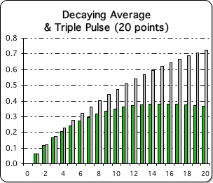
We can also view the Living Average in terms of its vertical components – moment-to-moment. In the graph at left we take a column view of both the Living Average and the Directional – the Living Algorithm's 1st and 2nd derivatives. Remember this is the result when the Living Algorithm digests a data stream consisting solely of ones, 20 to them to be specific. Accordingly, this graph is a snapshot of the first 20 data points of the Living Average and the Triple Pulse's Active Pulse, a.k.a. the Pulse of Attention, from a purely vertical perspective.
Living Average Combination: Data Bit's Contribution at each Moment in Time
Taking it the last step, we can combine the vertical and horizontal perspectives. We can further break the Living Average's horizontal components into vertical components as well. This differentiation is shown in the graph at the right. This is the featured graph. Each color rectangle represents each data byte's contribution to the Living Average at each moment in time. The data byte and the time increment are the fundamental units of the Living Algorithm System. Accordingly these rectangles cannot be broken down any further – for instance into partial moments and partial data bits. The Living Algorithm System does not deal in partials. According each color rectangle represents a quantum of information.
Color Rectangle: Specific Location = Specific Moment by Specific Data Bit
Each color rectangle can be characterized by a specific moment (in this case 0 through 20) and a specific data bit (also 0 through 20). For instance, the large blue rectangle at the bottom left of the graph represents the contribution of the 1st data bit to the Living Average at the 1st moment in time, while the yellow-orange rectangle at the upper right represents the contribution of the 20th data bit at the 20th moment in time. Each rectangle has a specific location in our graph.
Color Rectangle's Size Varies: Contribution of each Data Point at each Moment is Unique
The relative location of each data point's contribution to the common good can be specified precisely. However, it is visually evident that the contribution of each data point at each point in time varies widely, as is indicated by the relative size of the rectangles. In contrast to photons, the fundamental quanta of light, information quanta are variable in size. The thrust of the proofs that follow is to derive how these values are determined. Note: we are only talking about the height of the rectangle, as the bases are all the same quantity (1 time unit - the duration of time between each measurement.)
Algebraic Notation for Events
Events, Letters & Horizontal color strips
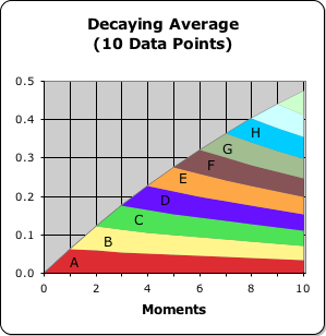
Before we can derive the equations that determine the values of the information quanta, we must first develop an algebraic notation that enables us to refer to individual quanta. Shown in the graph at right are the color strips that make up the Living Average of a data stream consisting of 10 ones. Let us define each of these color strips as an Event. Further, each Event has a letter associated with it. The 1st Event is always Event A, represented by the red strip; the 2nd Event is always Event B, the yellow strip: and so forth.
All of the Living Algorithm's Derivatives consist of an accumulation of Events
This labeling system applies to the Living Average, the Living Algorithm's 1st derivative. The Event labels also apply to the Directional, the Living Algorithm's 2nd derivative, as well as the Liminals, the Living Algorithm's higher derivatives. Each of the Living Algorithm's derivatives consists of an accumulation of layered Events.
Grid: the Derivative broken into vertical and horizontal components
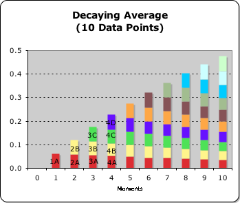
Now let us break these Events (the horizontal components) into their vertical components, as we did earlier. This deconstruction is shown in the graph at right. Because of the grid-like nature of the representation, we will refer to it as a Grid. As such, the graph is the Living Average Grid for a data stream consisting of 10 ones. The Living Average is the Living Algorithm's 1st derivative. Each Living Algorithm derivative has a unique Grid, as we shall see.
Info quantum identified by Event (a letter) and Moment (a number)
As mentioned, each of the colored rectangles in the Grid is a quantum of information. The horizontal component of each quantum is identified by a lettered Event. The vertical component of the each quantum is identified by a numbered Moment (the position in the data stream). Reiterating for clarity: each color rectangle (the info quanta) has a specific location in the Grid (the graph). Two features identify this location – the specific moment in the data stream (a number) and the specific Event (a letter). For instance, the 3rd red rectangle from the left is the 3rd moment of Event A (3A, as shown above).
Let's look at some specifics. Note that the red rectangles are identified by the letter A (Event A), the yellow rectangles by B (Event B), and so forth. The red rectangles represent the progressively diminishing influence of the first Event, A, on the Living Average at each moment in time. These moments are identified by numbers and correspond with N in the Living Algorithm. Accordingly, we can say that 4C refers to the contribution of Event C to the Living Average at the 4th moment in time (N = 4).
Alphanumeric schema like Excel, where letters represent a number
In the algebra that follows, we will employ this alphanumeric schema to refer to the individual info quanta. Excel employs a similar alphanumeric schema to label its spreadsheets – letters for columns and numbers for rows. Otherwise there are too many confusing numbers. The implied meaning is that the letters also have a number associated with them. For instance, in the Excel spreadsheet Column D is the 4th column and column AA is the 27th column. Similarly, Event D is the 4th event of the data stream.
Alphabetic Order
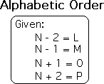
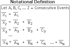
One last point: A feature of alphanumeric systems, such as those employed by Excel and us, is that numbers can be added to letters to obtain a letter. This feature is due to the fact that the letters stand for numbers. As an example A = 1, B = 2, and so forth. The alphabetic order reveals the number. As the last letter in the alphabet, Z = 26. We show an example at right.
Definitions: Events, Impact and Influences.
We've been speaking in generalities about Events. Let us define some terms.
Entry of data into Living Algorithm System initiates an Event
The Event begins when a data byte enters the Living Algorithm System. For instance, the entry of the 3rd data byte, X3, into the System initiates Event C. Note: due to alpha-numeric correspondence the 3rd data byte always initiates Event C, just as the 5th data byte always initiates Event E and the 1st data byte Event A. Every Event exerts an influence on all the Living Algorithm measures – the data stream derivatives – the Living Average, Directionals, etc.
Events: the Horizontal Component of the Grid
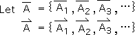
0.1 Let us put this analysis into an algebraic form. Let 'A bar' equal the data stream consisting of all the values in Living Average Event A. Let 'A arrow' equal the data stream consisting of all the values in Directional Event A. As mentioned, Events are the horizontal component of the 'Grid'.
Impacts and Influences
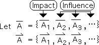
0.2 After the initial impact, each Event generates a declining influence upon successive moments. The declining size of the successive colored rectangles reflects this feature of Events. Note that these influences are discretized rather than continuous. Let us define the 1st info quantum of an Event as an 'impact' and the subsequent quanta as 'influences'. This differentiation (shown at right) is for algebraic purposes, as we shall see.
0.3 Reiterating for comprehension: each 'impact' and each 'influence' in the Living Average Grid represents a packet of info energy (an info quanta). The packet of energy is completely expended at its 'moment' in the 'Grid'. This quantum of info energy is consumed to influence the Decay Average at that 'moment'. Each quantum is associated with a lettered Event and a numbered moment (location in the data stream). The sum of Events at any particular moment yields the Living Average for that moment (shown at right). As mentioned, the columns in the graphic ‘Grid’ represent individual moments. As such, moments are the vertical component of the 'Grid'.
Summary Link
Now that we have established some algebraic definitions, we can begin to derive the dimensions of the individual quanta (colored rectangles) in our graph. For these derivations, check out the next article – Info Energy in the Living Average Grid.