Home Science Page Data Stream Momentum Directionals Root Beings The Experiment
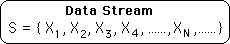
We will characterize a Data Stream, S, as an ordered data set, which is incomplete. Symbolically it is represented below.
Each of the Xs represents an ordered Data Point. X1 is the first point. X2 is the second point. XN is the Nth point. Although XN is shown as the last Data Point, there will always be another Data Point if it is a Data Stream because Data Streams are growing and hence incomplete.
Before beginning our discussion of the Derivatives of the Data Stream, we must distinguish between two types of Data Streams, the Continuous and Discontinuous Data Streams. A Continuous Data Streams begins from non-existence, hence has a defined history. Many naturally occurring Data Streams begin this way. A baby is born, the beginning of school, to begin playing an instrument. These streams emerge from non-existence. We will call these Continuous Data Streams, because there are no breaks in their history.
There are many other types of streams, which have existed for an indeterminate time before reaching consciousness. Their history is unknown. They emerge into consciousness from a prior existence. We will call these Discontinuous Data Streams because they begin abruptly with no continuous memory. Suppose someone has been reading for a long time, but decides at an abrupt point to start keeping track of his Reading Time, this would be an example of a Discontinuous Data Stream.
For the Continuous Data Stream, if the measured behavior or Action did not exist before the beginning, then the Action has a history, or non-history. This would be characterized by a string of zeros. The beginning of the Data Stream does not occur after a string of 0's. As an example: Before a baby is born, there is a string of zeros signifying no Baby time. We shall see that because of this all the Derivatives of the Data Stream are zero when the baby is born. Any new activity starts with a string of zeros, which is followed by something. So the first time someone plays the violin. This is not the first Data Point, I repeat not the first Data Point. The first Data Point in the series would be the first time that this organism did not play the violin.
The first Derivative of a Data Stream is the Decaying Average. Its equation is as follows.
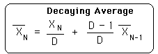
We do not need to know the value of N, the number of Data points, to determine the value of the Decaying Average. We only need to know the most recent Data Point, XN, and the previous Decaying Average. If XN is the first non-zero Data Point in a Continuous Data Stream, then the previous Decaying Average equals zero. We have had an indeterminate string of zeros preceding this point, with corresponding zeros for the Decaying Average. Hence the Decaying Average Equation is used immediately with a Continuous Data Stream. There is no confusion. *
At least not much. For the mathematicians in the crowd, who thrive on extreme examples, the beginning point, the Decay Factor, and the time interval must be designated, in order to determine if the string of zeros was long enough for us to immediately start using the Decaying Average equation above. Soon, when we look at Discontinuous Data Stream, we will discover that the string of zeros must make N greater than D for the Decaying Average equation to work immediately. The beginning point of a Continuous Data Stream is the first point at which the Action could have not existed. As an example, an organism is designated as starting with the beginning of the organism, itself. If we were talking about monthly time increments, the month a 25-year-old woman has a child would be the 300th Data Point. The Stream would have 299 months with no Baby Time followed by that first month of birth. (All the Deviations and Directionals go crazy, giving the mother an incredible rush.) If, however, the time increment were a year, then the year the mother had the child would be the 25th Data Point; the first 24 points would all be zeros. If, however, the time increment were a decade, then the decade the mother had the child would only be the 3rd Data Point; only the first 2 points would be zeros. Normally Decay factors are greater than 10. Hence the last series, based on a decade would have to be treated like a Discontinuous Data Stream. Read on to see why.
One last point before moving on. It must be cautioned that if the history prior to the 'beginning' of the Data Stream is not indeterminate, then the 'beginning' is a false one. Following is an example.
An example of the non-zero beginning of a Data Stream: If a person starts recording his hours of sleep at a certain point in his life, his Data Stream starts at that point, because the history before that point is indeterminate. It was not composed of a string of zeros, but was instead composed of an indeterminate Data Stream. Hence the first month that records are kept is the first Data point of the series. Activities with an indeterminate history begin with the first time period they are quantified. The Data Stream of beginning Activities begins with beginning of the organism itself, not with the beginning of the activity.
Let us generate the first derivative of our Discontinuous Data Stream, the Decaying Average. This is not as straightforward as it might seem. The general equation for the Decaying Average is listed below. This equation works quite well when N, the number of elements in the Data Stream is equal to or greater than D, the Decay Factor. When, however, N is less than D, then N must be substituted in the equation for D.

There are two reasons for this. The first is related to the actual possibility of generating the first term of the stream. Suppose D is 12 and we generate the Decaying Average the normal way, then the first average is indeterminate because there is not a previous, zeroth, average to generate it from. If there is no first term, there is no stream. Our study stops. While if because N < D, we substitute N for D in the equation then the previous, zeroth, average drops out and the first average becomes the first Data Point. See below.
Let us look at the first point in the Data Stream.
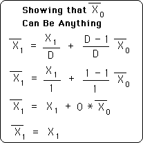
This shows two things. First it shows that the first data point is the first average. Second it shows that the zeroth average can be anything because it is multiplied by 0. The history before the first Data Point in the Data Stream is indeterminate or unknown. Similarly the history before the Big Bang is also indeterminate. We will look at more indeterminacy in a little bit.
We generate the second average of our Data Stream below.
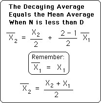
This illustrates the point that the Decaying Average equals the Mean Average of the whole set, until N, the number of Data Points in the Stream is greater than D, the Decay Factor. The Decaying Average was derived from the equation for the Mean Average. {See Decaying Averages Notebook.}
The second reason that N is substituted for D in the Decaying Average equation, when it is less than D, is of a more practical nature. If the Average is allowed to decay prematurely, i.e. when N < D, then the preceding values are given a disproportionate influence upon the new Average. Usually, i.e. when N > D, a Data Point will come in at 1/D of its value and then begins decaying at a rate of (D-1)/D. If we assign a value of '0' to the zeroth Average then we have already given our average a '0' weight of (D-1)/D, when the history is indeterminate. In our Sleep example, if the zeroth Average was given an arbitrary value of zero, D given a value of 10, our first point equaled 8 hours, then the average amount of hours of sleep per night, applying the general equation, would be equal to 0.8. Obviously nonsense.