Consolidating what we have learned
We've covered a lot of territory on our journey. Let's consolidate for retention.
Triple Pulse correspondences, Living Algorithm System & Data Stream Dynamics
In our exploration into the information-based nature of living systems, we've traversed multiple dimensions. In our 3 Notebooks, we’ve established: 1) patterns of correspondence between the Living Algorithm's Triple Pulse and Sleep; 2) the plausibility that the Living Algorithm System could be Life’s Operating System; and 3) that Data Stream Dynamics provides a possible causal mechanism behind the experimental correspondences. Currently, we're considering the role of Attention in this interconnected web that links the internal universe of information with the external physical universe.
Attention acts as intermediary between Living Algorithm & Life to prevent information overload.
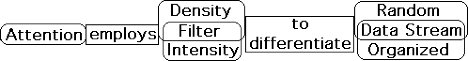
According to the Author’s model, Attention acts as the intermediary between living systems and the Living Algorithm. The Living Algorithm can digest any data stream and provide Life with a practical infinity of measures to describe each moment. But this is too much data - information overload – TMI. As the urge to actualize that permeates every level of the biological hierarchy, Life is only interested in information that is relevant to her quest. Attention is the tool Life employs to provide her with only the most relevant of the Living Algorithm's overly abundant information streams.
Attention focuses upon a data stream's intensity & density to censor random data streams.
What techniques does Attention employ to provide Life with only meaningful information? Remember, Life is Attention's boss and Attention's tool is the Living Algorithm. Life’s sensory apparatus takes in raw data streams from the environment. The Living Algorithm can digest each and every one. Her digestion process creates many measures. Attention only needs to focus upon two of these measures – a data stream's intensity and density. Both the intensity and density of random data streams are significantly lower than organized data streams. By focusing upon these measures, Attention is able to differentiate random from organized data streams.
Attention passes on Living Algorithm package as long as there is an Acceleration
Intensity and density are two forms of data stream acceleration. Accordingly, Life focuses Attention upon data stream acceleration to accomplish the primary task of censoring random data streams. This obsession with acceleration is at the expense of all the other measures, including data stream velocity. As long as a data stream has a significant acceleration, Attention passes on the entire Living Algorithm package to Life.
Where does Life come into the picture?
Censoring random data streams seems to be a primary function of the Attention/Living Algorithm synergy. Acting as a censor seems to be a relatively automatic process. Where does Life come into the picture?
How does Life regulate the Attention/Living Algorithm synergy?
As a mathematical system the Attention/Living Algorithm synergy is as mechanistic as a radio or computer. According to the Author’s model, Life’s freedom of choice lies in her ability to tweak the Attention/Living Algorithm System to provide her with the information she needs. Her experiences teach her the refinements.
What dials does Life turn to maximize her potentials?
But what mathematical features can Life play with? How does she regulate this System to better adjust to dynamic environmental circumstances? This adjustment is essential if she is to fulfill her sacred quest – the urge to actualize her potentials. Of course, this urge to self-actualize is quite different in her manifestation as a cell, a collection of cells, and the collection of a collection of cells that constitutes a human being. But the basic urge is the same. What mathematical dials can Life twist to get a better reading on the lay of the land – the information it contains?
To find out about the Living Algorithm’s Decay Factor, read on.
To provide a plausible answer to this question, we must introduce yet another member of the Living Algorithm’s menagerie – the Decay Factor. The Decay Factor is a major player in the Living Algorithm, and hence the Living Algorithm’s mathematical system. To understand the Decay Factor’s crucial role, check out the following article.
Living Algorithm Algebra: D, the Decay Factor
Living Algorithm Algebra Review
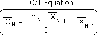
To get an understanding of the central importance of the Decay Factor in this study of Attention, let us first review the Living Algorithm's algebra – her basic elements – her permanent self. At right is the Living Algorithm, a.k.a the Cell Equation, in her simplest form.
Open System: Fresh Data enters with each Iteration
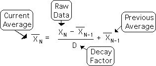
Reviewing the notation: the X without a hat is the Raw Data. We employ the N as a subscript to indicate that a new piece of data (info energy) enters the Living Algorithm System with each repetition (iteration) of her process. Like biological systems, the Living Algorithm System is open to influence from the external world. This is why she is an open system. Material systems are entirely different. They are closed systems where the matter/energy complex is indestructible.
Self-Referential System: Old Average employed to compute New Average
The X's with hats represent the Living Average. Note that they too have subscripts. This indicates their relative position in the data stream, with respect to each other and with respect to the Raw Data. A new Living Average is computed with each iteration (repetition) of the Living Algorithm process. The Living Algorithm employs the New Raw Data and the Old Living Average to compute the New Living Average. If the New Data Point is larger than the Old Average, the New Living Average is also larger and vice versa. Because the old is employed to generate the new, the process is self-referential. In similar fashion, biological systems, unlike material systems, must merge prior patterns with present input to create an updated version that will facilitate decision-making.
Decay Factor's sole function: Scaling factor of the Rate of Change
Besides the basic operations of arithmetic, the only remaining element in the Living Algorithm that is unaccounted for is D, the Decay Factor. D plays a significant part in the Living Algorithm process, but is unaffected by it. Because D's value is independent of the process, it has no subscript. D's sole function is to act as a scaling factor to the rate of change. The rate of change is the difference between the incoming Raw Data and the Past Average.
Decay Factor determines Rate of Decay, which determines Impact of Fresh Data on System
As implied by the name, D determines the rate of decay. When D’s value is large, the impact of the Fresh Data on the System is minimized. When D’s value is small, the impact is maximized. Accordingly, D, the Decay Factor, determines the impact of the incoming data upon the New Living Average. The slower the rate of decay, the less the impact of the New Data and vice versa. Decay Factor Up; Impact Down.
Unless refreshed, Living Average is constantly decaying
There are a few noteworthy points to this process that are worth mentioning. Without the introduction of fresh data into the System, the Living Average becomes successively smaller, eventually approaching zero. Each iteration (repetition) of the Living Algorithm process further erodes the value of the dying Living Average, until it reaches 'practical' zero. This is why D is deemed the Decay Factor.
Entropic Systems: Living Algorithm, heating, biological
Because of D, the Living Algorithm System is fundamentally an entropic system. Without the input of external energy, innate forces drive a heating system towards equilibrium. Similarly, without the input of external information, internal mechanisms drive the Living Algorithm System towards zero. In similar fashion, biological systems are subject to innate processes that lead to a constant state of decay. As such, each of these systems are entropic in nature.
Regenerative System: Possibility of Fresh Data
The possibility of regeneration with the introduction of fresh data balances this continual decay. Accordingly, we say that the Living Algorithm System is regenerative. Similarly, biological systems, unlike material systems, are in a constant state of regeneration in order to survive. This includes sensory input as well as sustenance (air, water, and food). In our article on learning, we argue that organisms also must regularly regenerate their information, as well.
Graphs: Decay Factor’s Range applied to a Single Point
The Decay Factor’s 5 pragmatic Sectors
Theoretically D, the Decay Factor, can be any positive whole number. Accordingly, D’s range is from 1 to infinity. Thus far in our investigations, the Living Algorithm’s Decay Factor, D, has been set at 16 to simplify matters. Although D can be any positive value, we can divide the Decay Factor’s continuum into 5 pragmatic sectors: instantaneous (D=1), volatile (D=2 through 9), stable (D=10 through 20), sedentary (D=20 through 50), and eternal (D greater than 50).
Graph: Data Bit = 1; D = 16
A. Decay Factor, D=16
B. Decay Factor in Stable Range
C. Decay Factor in Sedentary/Eternal Range
D. Decay Factor in the Volatile Range
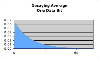
To better understand D's miraculous abilities, let us see what happens when the Living Algorithm digests a single piece (bit) of information from the Decay Factor’s multiple perspectives. Graph A visualizes what happens when the Living Algorithm digests a single data bit, the number 1, when the D is set at 16. The graph illustrates the successive impact of that piece of data once it enters the System. Notice that the impact is greatest when the data enters the system and then falls off. The shape of the curve would be identical no matter what the size of the data. (As mentioned, the Decay Factor determines the rate of decay, which determines the impact of New Data on the System.)
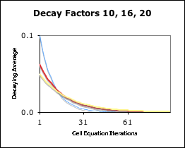
Graph: Stable – D = 10, 16, & 20
For comparison let's see what happens to the curve when the Decay Factor D is set at 10 and 20 - still in the stable range. This is illustrated in Graph B. The red line is identical to the curve in Graph A, (D = 16). The blue line visualizes the same process when D’s value is smaller (10). Notice how steep the descent of the blue line is in comparison to the red line. The blue line starts higher (.10 vs. .06) and ends more quickly (35 repetitions of the Living Algorithm process vs. 61). The smaller the Decay Factor is, the greater the impact of data on entry and the quicker it decays. Conversely the yellow line visualizes the same process with a greater D (20). Notice how flat the yellow line's descent is in comparison with the red line. The yellow line starts lower and ends more slowly. The greater the Decay Factor is, the smaller the impact of data on entry and the slower it decays.
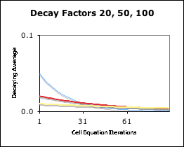
Graph: Sedentary to Eternal – D = 20, 50, & 100
Let's see what happens when the Decay Factor is even greater in magnitude. Graph C shows what happens to the data when D is in the sedentary to eternal range. The blue line is a visualization when D = 20, the red when D = 50, and the yellow line when D = 100. Notice as the Decay Factor gets higher that the horizontal line flattens out. This indicates a lower impact upon entry and a longer fade out time. In fact, the beginning and end values of the line get closer and closer in value as D’s value increases. As D approaches infinity (the true eternal state), these two values approach each other, as well.
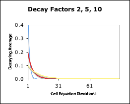
Graph: Volatile – D = 10, 5, & 2
Now let's see what happens when the Decay Factor is in the volatile range. Graph D illustrates this result. The Living Algorithm performs the same function as before (digesting a data stream consisting of a single 1 followed by 0s), but this time her Decay Factor is smaller. The yellow line represents the Living Algorithm’s digestive process when D= 10, the red line when D=5, and the blue line when D =2. Notice how the lines get steeper as the Decay Factor gets smaller. Their impact upon entry into the Living Algorithm System is greater, but they fade more rapidly.
Vertical Line: Instantaneous – D = 1
When D = 1, the instantaneous state, the curve turns into a vertical line. The impact is greatest because it happens all at once, yet there is no duration through time. It is evident that as D’s value gets smaller that the immediate impact is greater, but the lasting impact is reduced. Conversely, as D’s value gets larger the immediate impact is less, but the lasting impact is greater. As D approaches infinity, the curve turns into a horizontal line. The immediate impact and the lasting impact both approach zero.
Graphs: Decay Factor’s Range applied to an Individual Data Stream
We've just examined what happens when the Living Algorithm digests a single data point (1) with a range of Decay Factors. Now let us see what happens when the Living Algorithm digests an individual data stream with the same range of Decay Factors.
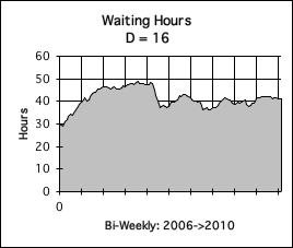
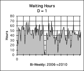
Data Stream: Bi-monthly Waiting Hours
A. Decay Factor = 16: Responsive
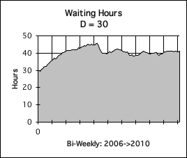
B. Decay Factor = 30: Sedentary
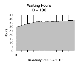
C. Decay Factor = 100: Eternal
Our data stream consists of the number of hours the Author spent waiting tables. These values were tabulated on a bi-monthly level from 2006 through 2010 – every time he got a paycheck. We chose this data stream for a specific reason. The variety of Decay Factors from volatile to sedentary can show off their specialties with this particular data stream. During this period two of the restaurants where he worked closed their doors - one due to the Recession of 2008-9. Plus he went through a physical/psychic breakdown at the beginning of 2008, which caused him to miss an abundance of work. Due to these factors, the data stream has moments of regularity mixed in with periods of abrupt starts and stops. Let's see how our Decay Factors reflect this turbulence.
D = 16, 30, 100: Responsive, Sedentary & Eternal
The Decay Factor is a mathematical feature of the Living Algorithm that determines how quickly the data’s impact decays after entering the System. In all of our prior articles we have employed a Decay Factor of 16. Graph A is a visualization of the Living Average when D = 16, the responsive range. The information in the graph is straightforward. It clearly shows that our Waiter worked nearly 50 hours each bimonthly pay period for the first few years. After a few dips, his average dropped to about 40 hours per pay period. Although Graph A indicates that the amount of time he worked declined, it doesn’t really indicate the turbulence that our Waiter went through.
When the Decay Factor rises to 30 (Graph B), the curve is not as responsive to the data. The highs aren't as high; the lows not as low; and the dips aren't as pronounced. This is why we say that a Decay Factor of 30 is in the sedentary range.
When the Decay Factor rises further to 100 (Graph C), the curve almost smoothes out into a straight line. It rises gradually from a low starting point to a low ending point. This is why we refer to this Decay Factor as being in the eternal range.
D = 10, 2, 1: Responsive, Volatile & Instantaneous
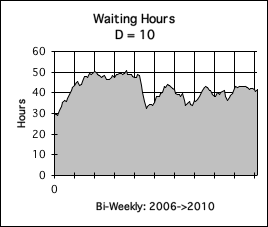
D. Decay Factor = 10: Sensitive
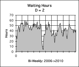
E. Decay Factor = 2: Volatile
F. Decay Factor = 1: Instanteous
Now let us see what happens to our graph when the Decay Factor gets smaller and smaller. The Decay Factor, D, is an element in the Living Algorithm that determines how quickly the data decays once it enters the System. The lower the value of D, the more rapidly the data’s impact decays. This leads to graphs that are more responsive to the data, When the Living Average dial is turned low enough the graphs response in more volatile. Graph D shows what happens when D = 10. Notice that the curve has greater definition than the prior curves. The highs are a little higher, the lows a little lower, and the dips far more pronounced. This is the Decay Factor that the Author employed when he first discovered the Living Average. This was in part due to the ease of computation and partially due to the sensitivity of the Decay Factor.
Let's see what happens when the Decay Factor is reduced even further. Graph E is a visualization of the Living Average of the same data stream, but when the Decay Factor is 2. Notice how jagged the curve is. This indicates the variability in the hours worked. The dips are much more pronounced. As is evident, graphs with lower Decay Factors reveal individual details more clearly. This is why we call this the volatile range. However, Decay Factors in the volatile range do not indicate the overall trends that are revealed by graphs with higher rates of decay.
Our final graph (Graph F) is a visualization of the Living Average of the same data stream when the Decay Factor = 1. This is a picture of the raw data. This is why we refer to it as the instantaneous range. The Data makes a complete impact when it enters the System and doesn't decay at all. Notice how great the range of hours worked is: from 0 to 80 hours per pay period. Some of the trends are obscured in the turbulence of the data, but the dips are clearly indicated (when he was out of work due to illness, and then unemployment).
Instantaneous perspective provides no context.
Viewed from the instantaneous perspective, the raw data provides an abundance of information, but obscures overall trends. To understand the context of the current moment, the instantaneous perspective is almost useless. The instantaneous perspective is so localized that it provides no relative context – no relation to the preceding data points in the stream. The Decay Factor must be greater than 1 to provide information that gives continuity to the flow of data.
Graph: All Decay Factors together for easy comparison
Below is a graph that visualizes the Living Average of the same data stream when digested by the same Living Algorithm but with different Decay Factors. We show them all together for an easy comparison.
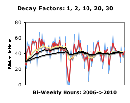
In general, the smaller the Decay Factor, the more volatile the information; and the greater the Decay Factor, the more sedentary the information. Of course there is a range of Living Averages in the middle that provide responsive and sensitive information. But as we shall see shortly, each level of the Decay Factor has an importance that our brain exploits for different reasons.
The nature of the linkage between Attention and the Living Algorithm’s Decay Factor?
It is evident that the Decay Factor is an important element of the Living Algorithm. The Decay Factor seems to be the dial that regulates the relative intensity of the Living Algorithm’s output. What is the nature of the linkage between Attention and the Living Algorithm’s Decay Factor?
We certainly don't know. To discover the nature of this interesting linkage, check out the next chapter – Posner's Attention Model & the Decay Factor.
To better assimilate this intriguing information, check out Life’s perspective on this unusual article. See why Life wonders about her role.