Section Headings
Origination of Basic Living Algorithm
Data Energy: Kinetic & Potential
A Single Data Point: Mathematics of Kinetic Energy
A Single Data Point: Mathematics of Potential Energy
Multiple Data Points: Mathematics of Data Energy
Synopsis
The Living Algorithm (LA), the mathematical foundation of our Theory of Attention generates a system. This article offers some mathematical derivations regarding the nature of Kinetic and Potential Energy in the LA's system. Each iteration of the LA's process integrates new data into the system. Each new data point can be viewed as a type of energy – deemed Data Energy. When it enters the system, part of the Data Energy is consumed as Kinetic Energy. This energy is employed to change or maintain the state of the system. The remainder of the original Data Energy is stored as Potential Energy. A portion of this Potential Energy is consumed as Kinetic Energy with each iteration of the LA's computational process. After enough iterations, the original Data Energy is completely consumed, at least for all practical purposes. However, if new Data Energy continues to enter the system, the Potential Energy accumulates. The LA’s computational process is unable to keep up. The system requires downtime to completely utilize the accumulating Potential Energy. Mathematical downtime is when the data stream's content equals zero. According to our Theory of Attention, this mathematical process is related to the necessity of Sleep and our limited Attention span.
Origination of Basic Living Algorithm
A1. Let us begin this discussion with the origination of the most basic form of the Living Algorithm (LA), a.k.a. the Decaying Average. Following is the equation for the Mean Average. All the members of the set are added up and then divided by the number of elements, N, in the set.
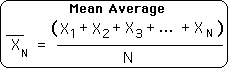
A2. Because I was exploring the nature of ongoing data streams, I needed an expression for a running average. Data streams are ordered and so each piece of data has a subscript to indicate its position in the data stream. Let XN denotes the most recent piece of data. Following is the expression for the Mean Average when an additional piece of data is added to the original set.
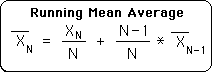
A3. I was interested in the nature of most recent moment in the data stream, not the entire data set. Because N grew with each new piece of data, the average became increasingly sedentary, hence uninteresting. To solve this problem, I simply substituted D, a fixed constant, for N, the number of elements in the set in the Mean Average formula above.
For reasons delineated elsewhere, D was deemed the Decay Factor. As a subscript in the Decaying Average formula, N represents the position in the data stream or the number of repetitions of the Living Algorithm's computational process.
D has major advantages in terms of characterizing the ongoing nature of data streams, my primary interest. These included computational ease in the days before computers were readily available. More importantly, as D remains the same, recent pieces of data have more weight, while still taking past data into account.
Because of its relationship to the Mean Average and because it contained the Decay Factor, the above equation was deemed the Decaying Average. After many decades of study and derivations, I came to realize that this simple algorithm could be applied to itself to produce the higher derivatives as well. Due to this generative capacity, the general equation was originally named the Cell Equation.
Much later, I uncovered many patterns of correspondence between these data stream derivatives and living systems, specifically Human Attention. Due to this intimate relationship with Life, I changed the name of the general process to the Living Algorithm. The Decaying Average is the most basic form of the Living Algorithm.
A4. Before leaving this section, let us write the Basic Living Algorithm (A3) in a more convenient form. The coefficient of the final expression is a simple function of D, the Decay Factor. Because of its importance, we will give this coefficient its own name and letter – S, the Scaling Factor. S is defined below. To facilitate the coming proofs, it is written in 2 forms.
![]()
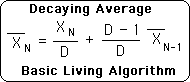
A5. Substituting S, the Scaling Factor, in our original equation (A3) yields the following result. In words, to obtain the current Decaying Average: 1) divide the current data point by the Decay Factor, D; 2) multiply the prior Decaying Average by the Scaling Factor, S; 3) then add these 2 quantities.
![]()
The Decaying Average is the first derivative of the data stream. This same algorithm, i.e. Living Algorithm, also produces the higher derivatives. The Decaying Average is the only focus of this discussion.
Data Energy: Kinetic & Potential
B1. The LA is an iterative function, i.e. based upon a repetitive process. Further, the LA is open, rather than closed, to external information. With each iteration, a new data point (XN) enters the LA’s System of Decaying Averages. Let the value of this data point represent the total Data Stream Energy entering the mathematical System at moment N. There could be energy from prior data points and future data points could add more energy. XN represents the total energy entering the System on the Nth Iteration of the LA’s computational process.
Let XN = Total Data Energy entering System on Nth Iteration of LA Process
B2. The sole purpose of this energy is to change or maintain the previous Decaying Average, i.e. the state of System. The effort to change the System is mathematical work. The work of changing the System occurs in stages, rather than instantaneously. The LA's computational process utilizes part of the XN's total energy and stores the remainder. Let us represent the portion of the total energy that does work with a K, as it represents kinetic, or working, Data Energy. Because it does work, it is consumed.
Let K = Kinetic Data Energy
B3. Let us represent the portion of total energy that is stored with a U, as it represents potential energy that will be converted to kinetic energy at a later date. In fact, as we shall see, with each repetition of the LA's computational process, part of this potential energy is converted to kinetic energy.
Let U = Potential Data Energy
B4. Just as with traditional systems of energy, the total energy equals the sum of the kinetic and potential energy.
![]()
B5. Because the total amount of energy is fixed, changes in kinetic energy are matched by equal and opposite changes in potential energy.
![]()
Because part of the Data Energy is stored and only used up gradually, both the amount of working (kinetic) energy, K, and the amount of stored (potential) energy, U, from the original energy lessens with each iteration.
A Single Data Point: Mathematics of Kinetic Energy
C1. Let us look at this exchange of Data Energy from an algebraic perspective. We begin with the Basic Living Algorithm, a.k.a. the Decaying Average (A3) .
![]()
C2. When our general data point, XN, first enters the System, it has had no prior influence on the second term in the expression. Its sole impact on current Decaying Average comes from the 1st term, i.e. XN/D. Let K1 equal the amount of kinetic energy that works to change or maintain the Decaying Average on the first iteration due to XN. The subscript indicates the number of iterations after our data point, XN, entered the System. (A subscript of 0 indicates that our data point has not yet entered the System.)
![]()
C3. A new data point, XN+1, enters the System on the next repetition of the LA's computational process. The prior data point, XN, the one that interests us, exerts no influence upon the 1st term in the expression.
![]()
C4. The 2nd term can be broken into 2 parts with a simple substitution of C1. As before, prior data points determine the value of the 2nd term of this expression.
![]()
C5. XN's sole impact upon the new Decaying Average comes from the 1st term. Its initial impact (C2) is scaled back by S. K2 is the amount of kinetic energy from XN's total energy that is consumed doing work to change or maintain the new Decaying Average on the 2nd iteration.
![]()
C6. On the third iteration, the same reasoning holds. XN exerts no influence upon the 1st term and its prior impact on the 2nd term is again scaled back by S from its prior influence (C4). K3 is the kinetic energy from XN that is consumed doing work on the 3rd iteration.
![]()
C7. Generalizing this pattern yields the following result.
![]()
C8. Because S is less than 1, zero is the limit of this process as M approaches ∞. With each iteration, the kinetic energy doing work shrinks, actually approaching 0. In other words, the total energy is eventually used up, consumed, at least for all practical purposes. (In contrast to physical systems, Data Energy is not conserved.)
![]()
C9. If we added up all of the kinetic energy that was employed after the original entry into the System, the sum would equal the original total Data Energy (XN). (Proved elsewhere.)
![]()
Summarizing our results, the initial impact of our data point upon the Decaying Average is the total energy divided by the Decay Factor (XN/D). Each successive iteration scales back this impact by S, the Scaling Factor. This process eventually consumes the entire amount of Data Energy (XN) that originally entered the System.
A Single Data Point: Mathematics of Potential Energy
D1. Recall that our single data point (XN) represents the total Data Energy as it enters the Living Algorithm System. Upon entry, the LA's computational process employs part of the energy to do the work of changing or maintaining the Decaying Average. K1 represents this initial expenditure of kinetic energy. The remainder of the information energy is stored as potential energy, U1. The total amount of energy is the sum of the initial kinetic energy and the initial potential energy.
![]()
D2. In other words, the potential energy is the difference between the total energy and the amount of energy that has been expended.
![]()
D3. Substituting for K1 from expression C2 in the preceding proof yields the following result. In words, the remaining potential energy equals the total amount of energy after it has been scaled once.
![]()
D4. The potential energy after the second iteration, U2, is the difference between the total energy that entered the system, XN, and the total amount of energy that has been expended, i.e. the sum of the initial kinetic energy, K1, and the kinetic energy that has done work in the second iteration, K2.
![]()
D5. Substituting the appropriate expressions from the preceding proof (C2 and C5) yields the following equation. We then perform some simple algebraic manipulations.
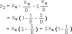
D6. Combining terms yields the following equation. In words, the remaining potential energy after two iterations, U2, equals the total amount of energy (XN) after it has been scaled twice, S2.
![]()
D7. The amount of potential energy remaining in the system after the 3rd iteration, U3, equals the difference between the total amount of energy (XN) and the sum of the energy that has been expended in all 3 iterations, i.e. the first 2 iterations and the current one.
![]()
D8. The first half of the equation's right hand side is simply U2, the remaining potential energy after the 2nd iteration. Expression C5 from the prior proof provides us with the kinetic energy that is consumed in the 3rd iteration, K3. Substituting these 2 terms in the prior equation yields the following result.
![]()
D9. Factoring out the common terms yields the following.
![]()
D10. The expression on the right hand side of the above equation is another version of the scaling factor, S. This provides us with a simplified expression for the remaining potential energy after the 3rd iteration. In words, the potential energy after three iterations, U3, equals the total amount of energy (XN) after it has been scaled three times, S3.
![]()
D11. This simple pattern can be repeated indefinitely to yield the following result. In words, the potential energy after M iterations, UM, equals the total amount of energy (XN) after it has been scaled M times, SM.
![]()
D12. Because the Scaling Factor, S, equals 1-1/D, it is less than 0. As such, each time S is multiplied by itself, the total gets smaller. Due to this self-multiplication, it shrinks logarithmically (very quickly) rather than arithmetically (slowly). As the following expression shows, the limit of this expression as M approaches infinity is zero. In other words, the potential energy is used up for all practical purposes after a finite number of repetitions of the Living Algorithm's computational process.
![]()
Summarizing our results: When Data Energy as represented by a single data point (XN) enters the Living Algorithm System, its total energy is split into kinetic and potential energy. The kinetic energy, K, is consumed doing work to change or maintain the System's state and the potential energy, U, is stored. With each subsequent iteration, a fraction of the potential energy is converted to kinetic energy, which is consumed. Because this is a relatively quick logarithmic process, all the potential energy is eventually converted into kinetic energy, at least for all practical purposes. The remaining amount of potential energy is negligible. In other words, after a finite number of repetitions, virtually the entire amount of original energy (XN) is consumed doing work to change or maintain the System.
Multiple Data Points: Mathematics of Data Energy
Our prior analysis focused upon what happens to a single data point, XN, when it enters the LA System. The computational process divides the Data Energy into kinetic energy that does work now and potential energy that is eventually converted to kinetic energy that does work later. Now let us examine what happens when a second data point enters the system.
E1. First our notation: the first data point is X1; the second data point is X2; N is the number of iterations of the LA's process. Both data points represent Data Energy. The first iteration divides X1's energy into kinetic and potential energy. The exact proportions are shown in the preceding proofs.
E2. The second iteration operates upon the Data Energies of both data points. Kinetic energy from both points is employed to change or maintain the state of the System. U2 is the amount of potential energy that remains after the 2nd iteration. U2 is the sum of the remaining potential energy from X1 (provided by D6) and the potential energy from the 2nd data point, X2, (provided by D3). While the potential energy from the 1st data point is shrinking, new potential energy from 2nd data point has been added to the System.
![]()
E3. On the 3rd iteration, a new data point (X3) with additional Data Energy enters the System. While the potential energy from the prior points is scaled back, new potential energy enters the System. If the data points are equal, the potential energy continues to grow.
![]()
E4. On the Mth iteration, a new data point (XM) with yet more Data Energy enters the System. In similar fashion, the potential energy of the Mth interation, UM, includes the scaled back potential energy from the prior iteration plus the fresh potential energy from the new data point.
![]()
If each of the data points is equal, the total potential energy increases with each repetition of the process. It is evident that the Living Algorithm can't keep up with the incoming energy. Although kinetic energy is consumed doing work to change or maintain the System, the potential energy continues to accumulate with each iteration. To completely consume the total energy entering the System, the Living Algorithm requires some downtime. No more Data Energy must enter the System to allow the LA to convert the accumulating potential energy into kinetic energy. If the total amount of potential energy is to be consumed as kinetic energy, the incoming data must be a string of 0s.
Data Energy is certainly a curious concept. How can raw data have energy? If this system had no connection with empirical reality, it would remain a mere oddity with very little significance. However, the Living Algorithm's mathematical processes seem to be intimately tied to Human Attention and the notion of Data Energy is linked to sleep.